- 浏览: 1664062 次
- 性别:

- 来自: 北京
-

文章分类
- 全部博客 (405)
- C/C++ (16)
- Linux (60)
- Algorithm (41)
- ACM (8)
- Ruby (39)
- Ruby on Rails (6)
- FP (2)
- Java SE (39)
- Java EE (6)
- Spring (11)
- Hibernate (1)
- Struts (1)
- Ajax (5)
- php (2)
- Data/Web Mining (20)
- Search Engine (19)
- NLP (2)
- Machine Learning (23)
- R (0)
- Database (10)
- Data Structure (6)
- Design Pattern (16)
- Hadoop (2)
- Browser (0)
- Firefox plugin/XPCOM (8)
- Eclise development (5)
- Architecture (1)
- Server (1)
- Cache (6)
- Code Generation (3)
- Open Source Tool (5)
- Develope Tools (5)
- 读书笔记 (7)
- 备忘 (4)
- 情感 (4)
- Others (20)
- python (0)
最新评论
-
532870393:
请问下,这本书是基于Hadoop1还是Hadoop2?
Hadoop in Action简单笔记(一) -
dongbiying:
不懂呀。。
十大常用数据结构 -
bing_it:
...
使用Spring MVC HandlerExceptionResolver处理异常 -
一别梦心:
按照上面的执行,文件确实是更新了,但是还是找不到kernel, ...
virtualbox 4.08安装虚机Ubuntu11.04增强功能失败解决方法 -
dsjt:
楼主spring 什么版本,我的3.1 ,xml中配置 < ...
使用Spring MVC HandlerExceptionResolver处理异常
Introduction
The problem of finding the Lowest Common Ancestor (LCA) of a pair of nodes in a rooted tree has been studied more carefully in the second part of the 20th century and now is fairly basic in algorithmic graph theory. This problem is interesting not only for the tricky algorithms that can be used to solve it, but for its numerous applications in string processing and computational biology, for example, where LCA is used with suffix trees or other tree-like structures. Harel and Tarjan were the first to study this problem more attentively and they showed that after linear preprocessing of the input tree LCA, queries can be answered in constant time. Their work has since been extended, and this tutorial will present many interesting approaches that can be used in other kinds of problems as well.
Let's consider a less abstract example of LCA: the tree of life. It's a well-known fact that the current habitants of Earth evolved from other species. This evolving structure can be represented as a tree, in which nodes represent species, and the sons of some node represent the directly evolved species. Now species with similar characteristics are divided into groups. By finding the LCA of some nodes in this tree we can actually find the common parent of two species, and we can determine that the similar characteristics they share are inherited from that parent.
Range Minimum Query (RMQ) is used on arrays to find the position of an element with the minimum value between two specified indices. We will see later that the LCA problem can be reduced to a restricted version of an RMQ problem, in which consecutive array elements differ by exactly 1.
However, RMQs are not only used with LCA. They have an important role in string preprocessing, where they are used with suffix arrays (a new data structure that supports string searches almost as fast as suffix trees, but uses less memory and less coding effort).
In this tutorial we will first talk about RMQ. We will present many approaches that solve the problem -- some slower but easier to code, and others faster. In the second part we will talk about the strong relation between LCA and RMQ. First we will review two easy approaches for LCA that don't use RMQ; then show that the RMQ and LCA problems are equivalent; and, at the end, we'll look at how the RMQ problem can be reduced to its restricted version, as well as show a fast algorithm for this particular case.
Notations
Suppose that an algorithm has preprocessing time f(n) and query time g(n). The notation for the overall complexity for the algorithm is <f(n), g(n)>.
We will note the position of the element with the minimum value in some array A between indices i and j with RMQA(i, j).
The furthest node from the root that is an ancestor of both u and v in some rooted tree T is LCAT(u, v).
Range Minimum Query(RMQ)
Given an array A[0, N-1] find the position of the element with the minimum value between two given indices.

Trivial algorithms for RMQ
For every pair of indices (i, j) store the value of RMQA(i, j) in a table M[0, N-1][0, N-1]. Trivial computation will lead us to an <O(N3), O(1)> complexity. However, by using an easy dynamic programming approach we can reduce the complexity to <O(N2), O(1)>. The preprocessing function will look something like this:
  void process1(int M[MAXN][MAXN], int A[MAXN], int N)
  {
      int i, j;
      for (i =0; i < N; i++)
          M[i][i] = i;
      for (i = 0; i < N; i++)
          for (j = i + 1; j < N; j++)
              if (A[M[i][j - 1]] < A[j])
                  M[i][j] = M[i][j - 1];
              else
                  M[i][j] = j;
  }
This trivial algorithm is quite slow and uses O(N2) memory, so it won't work for large cases.
An <O(N), O(sqrt(N))> solution
An interesting idea is to split the vector in sqrt(N) pieces. We will keep in a vector M[0, sqrt(N)-1] the position for the minimum value for each section. M can be easily preprocessed in O(N). Here is an example:
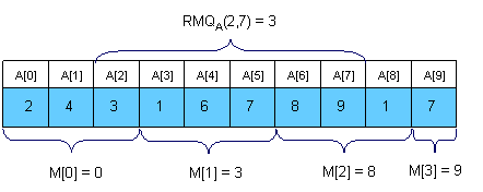
The main advantages of this approach are that is to quick to code (a plus for TopCoder-style competitions) and that you can adapt it to the dynamic version of the problem (where you can change the elements of the array between queries).
Sparse Table (ST) algorithm
A better approach is to preprocess RMQ for sub arrays of length 2k using dynamic programming. We will keep an array M[0, N-1][0, logN] where M[i][j] is the index of the minimum value in the sub array starting at i having length 2j. Here is an example:
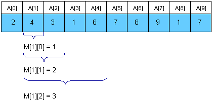
For computing M[i][j] we must search for the minimum value in the first and second half of the interval. It's obvious that the small pieces have 2j - 1 length, so the recurrence is:

The preprocessing function will look something like this:
  void process2(int M[MAXN][LOGMAXN], int A[MAXN], int N)
  {
      int i, j;

  //initialize M for the intervals with length 1
      for (i = 0; i < N; i++)
          M[i][0] = i;
  //compute values from smaller to bigger intervals
      for (j = 1; 1 << j <= N; j++)
          for (i = 0; i + (1 << j) - 1 < N; i++)
              if (A[M[i][j - 1]] < A[M[i + (1 << (j - 1))][j - 1]])
                  M[i][j] = M[i][j - 1];
              else
                  M[i][j] = M[i + (1 << (j - 1))][j - 1];
  }
Once we have these values preprocessed, let's show how we can use them to calculate RMQA(i, j). The idea is to select two blocks that entirely cover the interval [i..j] and find the minimum between them. Let k = [log(j - i + 1)]. For computing RMQA(i, j) we can use the following formula:

So, the overall complexity of the algorithm is <O(N logN), O(1)>.
Segment trees
For solving the RMQ problem we can also use segment trees. A segment tree is a heap-like data structure that can be used for making update/query operations upon array intervals in logarithmical time. We define the segment tree for the interval [i, j] in the following recursive manner:
Notice that the height of a segment tree for an interval with N elements is [logN] + 1. Here is how a segment tree for the interval [0, 9] would look like:
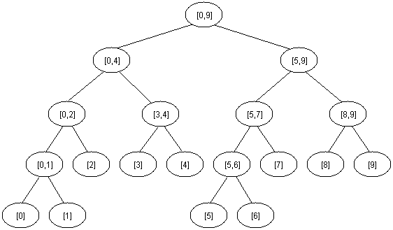
The segment tree has the same structure as a heap, so if we have a node numbered x that is not a leaf the left son of x is 2*x and the right son 2*x+1.
For solving the RMQ problem using segment trees we should use an array M[1, 2 * 2[logN] + 1] where M[i] holds the minimum value position in the interval assigned to node i. At the beginning all elements in M should be -1. The tree should be initialized with the following function (b and e are the bounds of the current interval):
  void initialize(intnode, int b, int e, int M[MAXIND], int A[MAXN], int N)
  {
      if (b == e)
          M[node] = b;
      else
       {
  //compute the values in the left and right subtrees
          initialize(2 * node, b, (b + e) / 2, M, A, N);
          initialize(2 * node + 1, (b + e) / 2 + 1, e, M, A, N);
  //search for the minimum value in the first and
  //second half of the interval
          if (A[M[2 * node]] <= A[M[2 * node + 1]])
              M[node] = M[2 * node];
          else
              M[node] = M[2 * node + 1];
      }
  }
The function above reflects the way the tree is constructed. When calculating the minimum position for some interval we should look at the values of the sons. You should call the function with node = 1, b = 0 and e = N-1.
We can now start making queries. If we want to find the position of the minimum value in some interval [i, j] we should use the next easy function:
int query(int node, int b, int e, int M[MAXIND], int A[MAXN], int i, int j)
{
int p1, p2;
You should call this function with node = 1, b = 0 and e = N - 1, because the interval assigned to the first node is [0, N-1].
It's easy to see that any query is done in O(log N). Notice that we stop when we reach completely in/out intervals, so our path in the tree should split only one time.
Using segment trees we get an <O(N), O(logN)> algorithm. Segment trees are very powerful, not only because they can be used for RMQ. They are a very flexible data structure, can solve even the dynamic version of RMQ problem, and have numerous applications in range searching problems.
Lowest Common Ancestor (LCA)
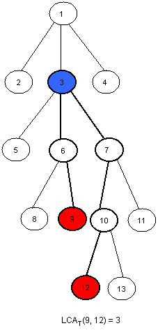
Given a rooted tree T and two nodes u and v, find the furthest node from the root that is an ancestor for both u and v. Here is an example (the root of the tree will be node 1 for all examples in this editorial):
An <O(N), O(sqrt(N))> solution
Dividing our input into equal-sized parts proves to be an interesting way to solve the RMQ problem. This method can be adapted for the LCA problem as well. The idea is to split the tree in sqrt(H) parts, were H is the height of the tree. Thus, the first section will contain the levels numbered from 0 to sqrt(H) - 1, the second will contain the levels numbered from sqrt(H) to 2 * sqrt(H) - 1, and so on. Here is how the tree in the example should be divided:
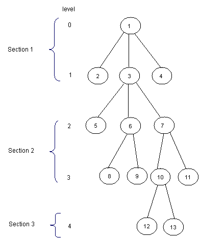
Now, for each node, we should know the ancestor that is situated on the last level of the upper next section. We will preprocess this values in an array P[1, MAXN]. Here is how P should look like for the tree in the example (for simplity, for every node i in the first section let P[i] = 1):

Notice that for the nodes situated on the levels that are the first ones in some sections, P[i] = T[i]. We can preprocess P using a depth first search (T[i] is the father of node i in the tree, nr is [sqrt(H)] and L[i] is the level of the node i):
  void dfs(int node, int T[MAXN], int N, int P[MAXN], int L[MAXN], int nr)  {
      int k;

  //if node is situated in the first
  //section then P[node] = 1
  //if node is situated at the beginning
  //of some section then P[node] = T[node]
  //if none of those two cases occurs, then
  //P[node] = P[T[node]]
      if (L[node] < nr)
          P[node] = 1;
      else
          if(!(L[node] % nr))
              P[node] = T[node];
          else
              P[node] = P[T[node]];

     for each son k of node
         dfs(k, T, N, P, L, nr);
  }
Now, we can easily make queries. For finding LCA(x, y) we we will first find in what section it lays, and then trivially compute it. Here is the code:
  int LCA(int T[MAXN], int P[MAXN], int L[MAXN], int x, int y)
  {
  //as long as the node in the next section of
  //x and y is not one common ancestor
  //we get the node situated on the smaller
  //lever closer
      while (P[x] != P[y])
          if (L[x] > L[y])
             x = P[x];
          else
     	       y = P[y];

  //now they are in the same section, so we trivially compute the LCA
      while (x != y)
          if (L[x] > L[y])
             x = T[x];
          else
             y = T[y];
      return x;
  }
This function makes at most 2 * sqrt(H) operations. Using this approach we get an <O(N), O(sqrt(H))> algorithm, where H is the height of the tree. In the worst case H = N, so the overall complexity is <O(N), O(sqrt(N))>. The main advantage of this algorithm is quick coding (an average Division 1 coder shouldn't need more than 15 minutes to code it).
Another easy solution in <O(N logN, O(logN)>
If we need a faster solution for this problem we could use dynamic programming. First, let's compute a table P[1,N][1,logN] where P[i][j] is the 2j-th ancestor of i. For computing this value we may use the following recursion:
![]()
The preprocessing function should look like this:
  void process3(int N, int T[MAXN], int P[MAXN][LOGMAXN])
  {
      int i, j;

  //we initialize every element in P with -1
      for (i = 0; i < N; i++)
          for (j = 0; 1 << j < N; j++)
              P[i][j] = -1;

  //the first ancestor of every node i is T[i]
      for (i = 0; i < N; i++)
          P[i][0] = T[i];

  //bottom up dynamic programing
      for (j = 1; 1 << j < N; j++)
         for (i = 0; i < N; i++)
             if (P[i][j - 1] != -1)
                 P[i][j] = P[P[i][j - 1]][j - 1];
  }
This takes O(N logN) time and space. Now let's see how we can make queries. Let L[i] be the level of node i in the tree. We must observe that if p and q are on the same level in the tree we can compute LCA(p, q) using a meta-binary search. So, for every power j of 2 (between log(L[p]) and 0, in descending order), ifP[p][j] != P[q][j] then we know that LCA(p, q) is on a higher level and we will continue searching for LCA(p = P[p][j], q = P[q][j]). At the end, both p and q will have the same father, so return T[p]. Let's see what happens if L[p] != L[q]. Assume, without loss of generality, that L[p] < L[q]. We can use the same meta-binary search for finding the ancestor of p situated on the same level with q, and then we can compute the LCA as described below. Here is how the query function should look:
  int query(int N, int P[MAXN][LOGMAXN], int T[MAXN],
  int L[MAXN], int p, int q)
  {
      int tmp, log, i;

  //if p is situated on a higher level than q then we swap them
      if (L[p] < L[q])
          tmp = p, p = q, q = tmp;

  //we compute the value of [log(L[p)]
      for (log = 1; 1 << log <= L[p]; log++);
      log--;

  //we find the ancestor of node p situated on the same level
  //with q using the values in P
      for (i = log; i >= 0; i--)
          if (L[p] - (1 << i) >= L[q])
              p = P[p][i];

      if (p == q)
          return p;

  //we compute LCA(p, q) using the values in P
      for (i = log; i >= 0; i--)
          if (P[p][i] != -1 && P[p][i] != P[q][i])
              p = P[p][i], q = P[q][i];

      return T[p];
  }
Now, we can see that this function makes at most 2 * log(H) operations, where H is the height of the tree. In the worst case H = N, so the overall complexity of this algorithm is <O(N logN), O(logN)>. This solution is easy to code too, and it's faster than the previous one.
Reduction from LCA to RMQ
Now, let's show how we can use RMQ for computing LCA queries. Actually, we will reduce the LCA problem to RMQ in linear time, so every algorithm that solves the RMQ problem will solve the LCA problem too. Let's show how this reduction can be done using an example:
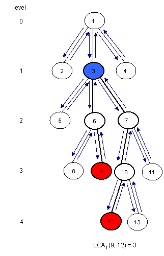
Notice that LCAT(u, v) is the closest node from the root encountered between the visits of u and v during a depth first search of T. So, we can consider all nodes between any two indices of u and v in the Euler Tour of the tree and then find the node situated on the smallest level between them. For this, we must build three arrays:
Assume that H[u] < H[v] (otherwise you must swap u and v). It's easy to see that the nodes between the first occurrence of u and the first occurrence of v areE[H[u]...H[v]]. Now, we must find the node situated on the smallest level. For this, we can use RMQ. So, LCAT(u, v) = E[RMQL(H[u], H[v])] (remember that RMQ returns the index). Here is how E, L and H should look for the example:
Notice that consecutive elements in L differ by exactly 1.
From RMQ to LCA
We have shown that the LCA problem can be reduced to RMQ in linear time. Here we will show how we can reduce the RMQ problem to LCA. This means that we actually can reduce the general RMQ to the restricted version of the problem (where consecutive elements in the array differ by exactly 1). For this we should use cartesian trees.
A Cartesian Tree of an array A[0, N - 1] is a binary tree C(A) whose root is a minimum element of A, labeled with the position i of this minimum. The left child of the root is the Cartesian Tree of A[0, i - 1] if i > 0, otherwise there's no child. The right child is defined similary for A[i + 1, N - 1]. Note that the Cartesian Tree is not necessarily unique if A contains equal elements. In this tutorial the first appearance of the minimum value will be used, thus the Cartesian Tree will be unique. It's easy to see now that RMQA(i, j) = LCAC(i, j).
Here is an example:

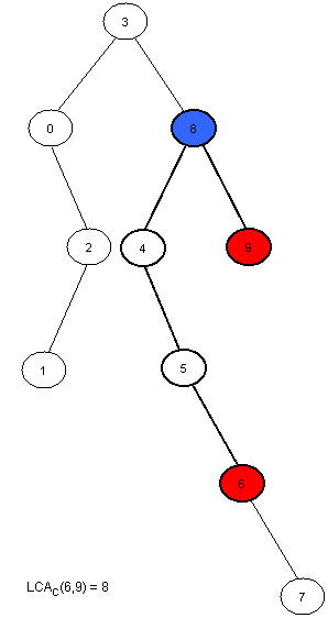
Now we only have to compute C(A) in linear time. This can be done using a stack. At the beginning the stack is empty. We will then insert the elements of A in the stack. At the i-th step A[i] will be added next to the last element in the stack that has a smaller or equal value to A[i], and all the greater elements will be removed. The element that was in the stack on the position of A[i] before the insertion was done will become the left son of i, and A[i] will become the right son of the smaller element behind him. At every step the first element in the stack is the root of the cartesian tree. It's easier to build the tree if the stack will hold the indexes of the elements, and not their value.
Here is how the stack will look at each step for the example above:
Step
Stack
Modifications made in the tree
0
0
0 is the only node in the tree.
1
0 1
1 is added at the end of the stack. Now, 1 is the right son of 0.
2
0 2
2 is added next to 0, and 1 is removed (A[2] < A[1]). Now, 2 is the right son of 0 and the left son of 2 is 1.
3
3
A[3] is the smallest element in the vector so far, so all elements in the stack will be removed and 3 will become the root of the tree. The left child of 3 is 0.
4
3 4
4 is added next to 3, and the right son of 3 is 4.
5
3 4 5
5 is added next to 4, and the right son of 4 is 5.
6
3 4 5 6
6 is added next to 5, and the right son of 5 is 6.
7
3 4 5 6 7
7 is added next to 6, and the right son of 6 is 7.
8
3 8
8 is added next to 3, and all greater elements are removed. 8 is now the right child of 3 and the left child of 8 is 4.
9
3 8 9
9 is added next to 8, and the right son of 8 is 9.
Note that every element in A is only added once and removed at most once, so the complexity of this algorithm is O(N). Here is how the tree-processing function will look:
void computeTree(int A[MAXN], int N, int T[MAXN])
An<O(N), O(1)> algorithm for the restricted RMQ
Now we know that the general RMQ problem can be reduced to the restricted version using LCA. Here, consecutive elements in the array differ by exactly 1. We can use this and give a fast <O(N), O(1)> algorithm. From now we will solve the RMQ problem for an array A[0, N - 1] where |A[i] - A[i + 1]| = 1, i = [1, N - 1]. We transform A in a binary array with N-1 elements, where A[i] = A[i] - A[i + 1]. It's obvious that elements in A can be just +1 or -1. Notice that the old value of A[i] is now the sum of A[1], A[2] .. A[i] plus the old A[0]. However, we won't need the old values from now on.
To solve this restricted version of the problem we need to partition A into blocks of size l = [(log N) / 2]. Let A'[i] be the minimum value for the i-th block in A andB[i] be the position of this minimum value in A. Both A and B are N/l long. Now, we preprocess A' using the ST algorithm described in Section1. This will takeO(N/l * log(N/l)) = O(N) time and space. After this preprocessing we can make queries that span over several blocks in O(1). It remains now to show how the in-block queries can be made. Note that the length of a block is l = [(log N) / 2], which is quite small. Also, note that A is a binary array. The total number of binary arrays of size l is 2l=sqrt(N). So, for each binary block of size l we need to lock up in a table P the value for RMQ between every pair of indices. This can be trivially computed in O(sqrt(N)*l2)=O(N) time and space. To index table P, preprocess the type of each block in A and store it in array T[1, N/l]. The block type is a binary number obtained by replacing -1 with 0 and +1 with 1.
Now, to answer RMQA(i, j) we have two cases:
Conclusion
RMQ and LCA are strongly related problems that can be reduced one to another. Many algorithms can be used to solve them, and they can be adapted to other kind of problems as well.
Here are some training problems for segment trees, LCA and RMQ:
SRM 310 -> Floating Median
http://acm.pku.edu.cn/JudgeOnline/problem?id=1986
http://acm.pku.edu.cn/JudgeOnline/problem?id=2374
http://acmicpc-live-archive.uva.es/nuevoportal/data/problem.php?p=2045
http://acm.pku.edu.cn/JudgeOnline/problem?id=2763
http://www.spoj.pl/problems/QTREE2/
http://acm.uva.es/p/v109/10938.html
http://acm.sgu.ru/problem.php?contest=0&problem=155
References
- "Theoretical and Practical Improvements on the RMQ-Problem, with Applications to LCA and LCE" [PDF] by Johannes Fischer and Volker Heunn
- "The LCA Problem Revisited" [PPT] by Michael A.Bender and Martin Farach-Colton - a very good presentation, ideal for quick learning of some LCA and RMQ aproaches
- "Faster algorithms for finding lowest common ancestors in directed acyclic graphs" [PDF] by Artur Czumaj, Miroslav Kowaluk and Andrzej Lingas
评论
(1)
/ \
(2) (7)
/ \ \
(3) (4) (8)
/ \
(5) (6)
一个nlogn 预处理,O(1)查询的算法.
Step 1:
按先序遍历整棵树,记下两个信息:结点访问顺序和结点深度.
如上图:
结点访问顺序是: 1 2 3 2 4 5 4 6 4 2 1 7 8 7 1 //共2n-1个值
结点对应深度是: 0 1 2 1 2 3 2 3 2 1 0 1 2 1 0
Step 2:
如果查询结点3与结点6的公共祖先,则考虑在访问顺序中
3第一次出现,到6第一次出现的子序列: 3 2 4 5 4 6.
这显然是由结点3到结点6的一条路径.
在这条路径中,深度最小的就是最近公共祖先(LCA). 即
结点2是3和6的LCA.
Step 3:
于是问题转化为, 给定一个数组R,及两个数字i,j,如何找出
数组R中从i位置到j位置的最小值..
如上例,就是R[]={0,1,2,1,2,3,2,3,2,1,0,1,2,1,0}.
i=2;j=7;
这个问题就是经典的RMQ问题.
这里介绍一个比较简单的方法O(nlogn)预处理,O(1)回答每个询问.
RMQ问题的预处理:
用一个数组d[i][j]表示数组R中,从i位置到i+2^j-1位置的最小值.
这个d[i][j]很容易dp得到.
d[i][j+1]=min{d[i][j],d[i+2^j][j]};
空间: O(nlogn) 时间: O(nlogn).
Step 4:
询问:
如果询问:从a到b里面最小的值..主要思路找两个长度是2^k的区间:
[a,a+2^k-1]及[b-1-2^k,b]把区间[a,b]覆盖掉. 这很容易做到的,
只要: 2^k*2>= |b-a|.
于是a到b里面的最小值 = min {d[a][k],d[b-2^k-1][k]}
发表评论
-
二分查找之变型题目
2010-10-24 12:40 2183二分查找算法在各个公司的笔试面试题大量出现,通常不是简单一眼就 ... -
一道笔试题(创新工厂)解法
2010-10-21 17:44 1892一个帖子http://www.iteye.com/topic/ ... -
[zz]大数据量,海量数据 处理方法总结
2010-08-27 22:24 2290大数据量的问题是很多面试笔试中经常出现的问题,比如baidu ... -
Trie and suffix array
2010-04-13 20:54 1945字典数Trie和后缀数组suffix array是处理字符串操 ... -
金币问题
2009-11-09 08:41 2060今年某公司的笔试题: 一个矩阵地图,每一个元素值代表金币数, ... -
楼梯问题
2009-11-09 08:19 1599hl给我的几道某公司的算法题: 1、 有个 100 级的 ... -
一道考察模拟乘法的题目
2009-11-07 22:37 1438今天hl和我讨论一道题目: 写道 整形数组如a={1,4, ... -
链表归并
2009-11-07 21:40 1056以前gx同学问的某某公司的笔试题,写一下练练(纯手写,没编译过 ... -
找出出现次数超过一半的数字
2009-11-07 21:23 1912hl同学问我一道这个题,想了一种方法,感觉还是不错的,只扫描一 ... -
有道难题以超低分晋级
2009-06-10 11:36 1598有道难题比赛居然晋级了,可以领到一个t-shirt。 -
逆序数/逆序数对
2009-06-09 23:17 3818逆序数是个常遇到的问题,主要有两种解法: O(n^2)的方法: ... -
有道难题topcoder
2009-05-31 23:55 2489今天做了有道topcoder的题目,也是第一次在topcode ... -
百度之星第一场题目
2009-05-31 00:03 3688由于不符合参赛条件,未能参加百度之星,看了题目还挺有意思,把题 ... -
一个对字符串很好的Hash函数ELFHHash
2009-05-03 21:41 2294#include<stdio.h> #defin ... -
最大流Ford-Fulkerson算法
2009-04-22 17:33 9731算法导论对最大流算法有很详细的介绍,今天实现了最大流Ford- ... -
大数/高精度加减乘除取模[收藏]
2009-04-16 19:38 5107#include <iostream> #i ... -
带重复数字的全排列
2009-04-16 18:58 3928上次gx同学问我一道又重复数字的全排列的问题,我当时用set保 ... -
差分约束系统
2009-04-15 16:00 3791(本文假设读者已经有以下知识:最短路径的基本性质、Bellma ... -
二分图匹配
2009-04-15 15:40 3753二分图最大匹配的匈牙利算法 二分图是这样一个图,它的顶点可以分 ... -
线段树
2009-03-24 10:58 1700把问题简化一下: 在自然数,且所有的数不大于30000的 ...


相关推荐
关于RMQ和LCA的关系的知识,如何用RMQ和LCA的转换
**RMQ(Range Minimum Query)与LCA(Lowest Common Ancestor)问题**是图论与数据结构领域中的两个重要概念,广泛应用于算法设计和优化。这篇由郭华阳所著的国家队论文深入探讨了这两个问题及其解决方案。 **RMQ...
3.郭华阳《RMQ与LCA问题》.ppt
**RMQ 与 LCA 问题的提出** RMQ(Range Minimum Query)问题是指在一个数组中,查询一段连续子序列的最小值。例如,给定一个数组 A[1...n],对于任意的 l 和 r (1 ≤ l ≤ r ≤ n),我们需要能够快速找到 A[l...r] ...
### RMQ与LCA问题及其相互关系 #### 引言 在算法领域,Range Minimum Query (RMQ) 和 Lowest Common Ancestor (LCA) 问题不仅因其自身的挑战性而受到关注,更因为它们在字符串处理、计算生物学以及其他复杂数据...
【RMQ(Range Minimal Query)】 RMQ,即范围最小值查询,是计算机科学中数据结构和算法设计的一个重要概念。它涉及到在一个数组或序列中寻找...通过学习和掌握RMQ和LCA,参赛者能够在竞赛中获得优势,提高解题能力。
算法学习
RMQ(Range Minimum/Maximum Query,区间最值查询)和LCA(Least Common Ancestor,最近公共祖先)是数据结构和算法中的重要概念,它们在解决实际问题中有着广泛的应用。下面将详细介绍这两种算法的基本概念、经典...
在ACM(国际大学生程序设计竞赛)中,RMQ(Range Minimal Query)和LCA(Least Common Ancestor)是两种常见的数据结构问题,通常出现在树形结构或数组中。 RMQ问题指的是在一个数组中,对给定区间进行最小值查询。...
该ppt讲了一种基于线段树的RMQ的ST算法问题和LCA算法,适合初学者用。
算法文档无代码RMQ&LCA问题提取方式是百度网盘分享地址
RMQ(Range Minimum Query,区间最小值查询)与LCA(Lowest Common Ancestor,最近公共祖先)是两种常见的算法问题,广泛应用于数据结构、图论以及计算机科学竞赛中。 RMQ问题通常涉及到在一个给定的线性序列A中,...
### RMQ与LCA:最近公共祖先解析及解法 #### 一、引言 在计算机科学领域,尤其是在算法设计中,“最近公共祖先”(LCA, Least Common Ancestor)和“区间最小值查询”(RMQ, Range Minimum Query)是两个非常重要...
倍增法介绍以及应用(RMQ、LCA) 倍增法是一种常用的算法思想,广泛应用于解决范围查询、最近公共祖先等问题。下面,我们将详细介绍倍增法的定义、应用以及优化方法。 倍增法定义 ---------- 倍增法是指每个数是...
如“重新审阅LCA问题”中所述,这将使用“范围最小查询”实现LCA。 已完成:天真RMQ,更快RMQ(使用nlogn稀疏表) 待办事项:执行±1 RMQ 天真的RMQ输出: (1(2(4..)(5..))(3(6..)(7..))) indexs : 0, 1, 2, 3,...
### LCA与RMQ问题详解 #### 一、问题描述 **LCA(Least Common Ancestors)** 和 **RMQ(Range Minimum Query)** 是数据结构和算法领域中两个非常重要的概念,它们各自解决了不同的问题,但在某些情况下可以互相转换...
LCA RMQ 最小公共祖先 区间最小值 LCA(Lowest Common Ancestor)和 RMQ(Range Minimum Query)是两种常见的数据结构算法问题。LCA 问题的目的是在一棵树中找到两个结点的最近公共祖先,而 RMQ 问题的目的是在一个...
在计算机科学领域,特别是数据结构和算法分析中,"LCA问题归约成RMQ求解"是一个重要的主题。LCA代表最远公共祖先(Least Common Ancestor),而RMQ代表范围最小值查询(Range Minimum Query)。这两个概念常用于树形...
【LCA(最近公共祖先)】 最近公共祖先(Lowest ...总的来说,LCA和RMQ都是数据结构和算法中的经典问题,它们在处理树形结构和数组区间查询时有着广泛的应用。掌握这些方法,对于解决类似问题能提供高效的解决方案。
在计算机科学领域,算法是解决问题的关键,而LCA(最近公共祖先)和RMQ(区间最值查询)是树形结构和数组处理中常见的两类问题。本文将详细介绍这两种算法及其高效解决方案。 首先,LCA(最近公共祖先)问题是在...