Probabilistic Data Structures for Web Analytics and Data Mining

https://highlyscalable.wordpress.com/2012/05/01/probabilistic-structures-web-analytics-data-mining/

 

Statistical analysis and mining of huge multi-terabyte data sets is a common task nowadays, especially in the areas like web analytics and Internet advertising. Analysis of such large data sets often requires powerful distributed data stores like Hadoop and heavy data processing with techniques like MapReduce. This approach often leads to heavyweight high-latency analytical processes and poor applicability to realtime use cases. On the other hand, when one is interested only in simple additive metrics like total page views or average price of conversion, it is obvious that raw data can be efficiently summarized, for example, on a daily basis or using simple in-stream counters.  Computation of more advanced metrics like a number of unique visitor or most frequent items is more challenging and requires a lot of resources if implemented straightforwardly. In this article, I provide an overview of probabilistic data structures that allow one to estimate these and many other metrics and trade precision of the estimations for the memory consumption. These data structures can be used both as temporary data accumulators in query processing procedures and, perhaps more important, as a compact – sometimes astonishingly compact – replacement of raw data in stream-based computing.

I would like to thank Mikhail Khludnev and Kirill Uvaev, who reviewed this article and provided valuable suggestions.

Let us start with a simple example that illustrates capabilities of probabilistic data structures:

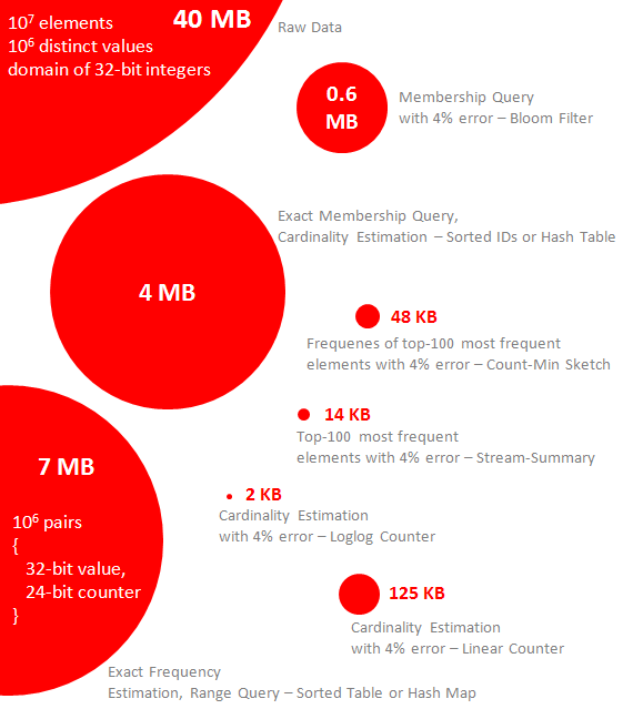
Let us have a data set that is simply a heap of ten million random integer values and we know that it contains not more than one million distinct values (there are many duplicates). The picture above depicts the fact that this data set basically occupies 40MB of memory (10 million of 4-byte elements). It is a ridiculous size for Big Data applications, but this a reasonable choice to show all structures in scale. Our goal is to convert this data set to compact structures that allow one to process the following queries:

• How many distinct elements are in the data set (i.e. what is the cardinality of the data set)?
• What are the most frequent elements (the terms “heavy hitters” and “top-k elements” are also used)?
• What are the frequencies of the most frequent elements?
• How many elements belong to the specified range (range query, in SQL it looks like  SELECT count(v) WHERE v >= c1 AND v < c2)?
• Does the data set contain a particular element (membership query)?

The picture above shows (in scale) how much memory different representations of the data set will consume and which queries they support:

• A straightforward approach for cardinality computation and membership query processing is to maintain a sorted list of IDs or a hash table. This approach requires at least 4MB because we expect up to 10^6 values, the actual size of the hash table will be even larger.
• A straightforward approach for frequency counting and range query processing is to store a map like (value -> counter) for each element. It requires a table of 7MB that stores values and counters (24-bit counters are sufficient because we have not more than 10^7 occurrences of each element).
• With probabilistic data structures, a membership query can be processed with 4% error rate (false positive answers) using only 0.6MB of memory if data is stored in the Bloom filter.
• Frequencies of 100 most frequent elements can be estimated with 4% precision using Count-Min Sketch structure that uses about 48KB (12k integer counters, based on the experimental result), assuming that data is skewed in accordance with Zipfian distribution that models well natural texts, many types of web events and network traffic. A group of several such sketches can be used to process range query.
• 100 most frequent items can be detected with 4% error (96 of 100 are determined correctly, based on the experimental results) using Stream-Summary structure, also assuming Zipfian distribution of probabilities of the items.
• Cardinality of this data set can be estimated with 4% precision using either Linear Counter or Loglog Counter. The former one uses about 125KB of memory and its size is linear function of the cardinality, the later one requires only 2KB and its size is almost constant for any input. It is possible to combine several linear counters to estimate cardinality of the corresponding union of sets.

A number of probabilistic data structures is described in detail in the following sections, although without excessive theoretical explanations – detailed mathematical analysis of these structures can be found in the original articles.  The preliminary remarks are:

• For some structures like Loglog Counter or Bloom filter, there exist simple and practical formulas that allow one to determine parameters of the structure on the basis of expected data volume and required error probability. Other structures like Count-Min Sketch or Stream-Summary have complex dependency on statistical properties of data and experiments are the only reasonable way to understand their applicability to real use cases.
• It is important to keep in mind that applicability of the probabilistic data structures is not strictly limited by the queries listed above or by a single data set. On the contrary, structures populated by different data sets can often be combined to process complex queries and other types of queries can be supported by using customized versions of the described algorithms.

Cardinality Estimation: Linear Counting

Let us start with a very simple technique that is called Linear Counting. Basically, a liner counter is just a bit set and each element in the data set is mapped to a bit. This process is illustrated in the following code snippet:

1 2 3 4 5 6 7 8

class LinearCounter {     BitSet mask = new BitSet(m) // m is a design parameter       void add(value) {         int position = hash(value) // map the value to the range 0..m         mask.set(position) // sets a bit in the mask to 1     } }

Let’s say that the ratio of a number of distinct items in the data set to m is a load factor. It is intuitively clear that:

• If the load factor is much less than 1, a number of collisions in the mask will be low and weight of the mask (a number of 1’s) will be a good estimation of the cardinality.
• If the load factor is higher than 1, but not very high, many different values will be mapped to the same bits. Hence the weight of the mask is not a good estimation of the cardinality. Nevertheless, it is possible that there exist a function that allows one to estimate the cardinality on the basis of weight (real cardinality will always be greater than weight).
• If the load factor is very high (for example, 100), it is very probable that all bits will be set to 1 and it will be impossible to obtain a reasonable estimation of the cardinality on the basis of the mask.

If so, we have to pose the following two questions:

• Is there a function that maps the weight of the mask to the estimation of the cardinality and how does this function look like?
• How to choose m on the basis of the expected number of the unique items (or upper bound) and the required estimation error?

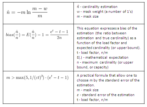
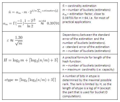
Both questions were addressed in [1]. The following table contains key formulas that allow one to estimate cardinality as a function of the mask weight and choose parameter m by required bias or standard error of the estimation:

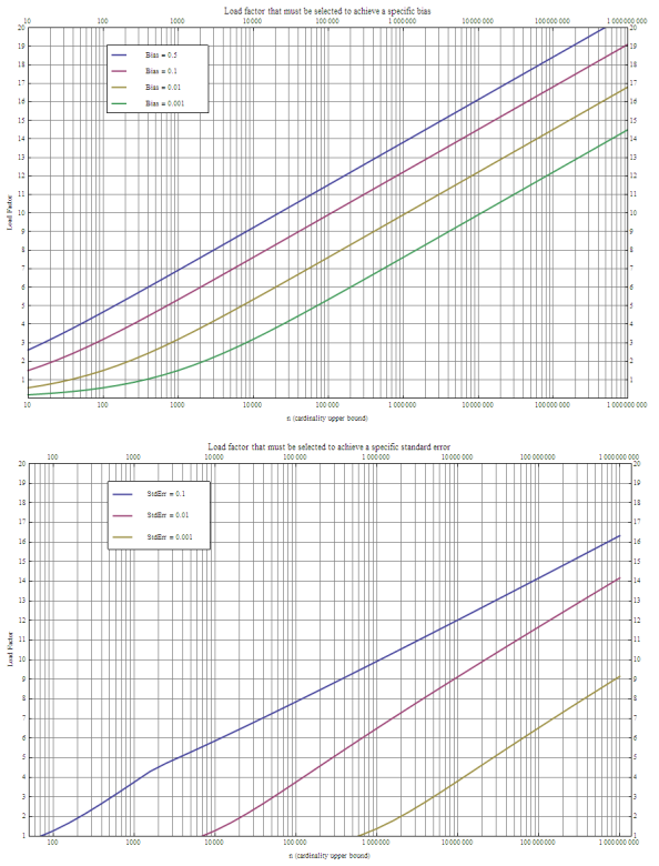
The last two equations cannot be solved analytically to express m or load factor as a function of bias or standard error, but it is possible to tabulate numerical solutions. The following plots can be used to determine the load factor (and, consequently, m) for different capacities.

The rule of thumb is that load factor of 10 can be used for large data sets even if very precise estimation is required, i.e. memory consumption is about 0.1 bits per unique value. This is more than two orders of magnitude more efficient than the explicit indexing of 32- or 64-bit identifiers, but memory consumption grows linearly as a function of the expected cardinality (n), i.e. capacity of counter.

It is important to note that several independently computed masks for several data sets can be merged as a bitwise OR to estimate the cardinality of the union of the data sets. This opportunity is leveraged in the following case study.

Case Study

There is a system that receives events on user visits from different internet sites. This system enables analysis to query a number of unique visitors for the specified date range and site. Linear Counters can be used to aggregate information about registered visitor IDs for each day and site, masks for each day are saved, and a query can be processed using bitwise OR-ing of the daily masks.

Cardinality Estimation: Loglog Counting

Loglog algorithm [2] is a much more powerful and much more complex technique than the Linear Counting algorithm. Although some aspects of the Loglog algorithm are pretty complex, the basic idea is simple and ingenious.

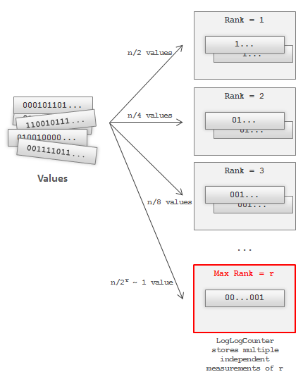
In order to understand principles of the Loglog algorithm we should start one general observation. Let us imagine that we hashed each element in the data set and these hashed values are presented as binary strings. We can expect that about one half of strings will start with 1, one quarter will start with 01, and so on. Let’s denote the number of the leading zeros as a rank. Finally, one or a few values will have some maximum rank r, as it shown in the figure below.

From this consideration it follows that 2^r can be treated as some kind of the cardinality estimation, but a very unstable estimation – r is determined by one or few items and variance is very high. However, it is possible to overcome this issue by using multiple independent observations and averaging them. This technique is shown in the code snippet below. Incoming values are routed to a number of buckets by using their first bits as a bucket address. Each bucket maintains a maximum rank of the received values:

1 2 3 4 5 6 7 8 9 10 11 12 13 14 15 16 17

class LogLogCounter {     int H           // H is a design parameter     int m = 2^k         // k is a design parameter     etype[] estimators = new etype[m] // etype is a design parameter       void add(value) {         hashedValue = hash(value)         bucket = getBits(hashedValue, 0, k)         estimators[bucket] = max(             estimators[bucket],             rank( getBits(hashedValue, k, H) )         )     }       getBits(value, int start, int end)     rank(value) }

This implementation requires the following parameters to be determined:

• H – sufficient length of the hash function (in bits)
• k – number of bits that determine a bucket, 2^k is a number of buckets
• etype – type of the estimator (for example, byte), i.e. how many bits are required for each estimator

The auxiliary functions are specified as follows:

• hash(value) – produces H-bit hash of the value
• getBits(value, start, end) – crop bits between start and end positions from the value and return an integer number that is assembled from this bits
• rank(value) – compute position of first 1-bit in the value, i.e. rank(1…b) is 1, rank (001…b) is 3, rank (00001…b) is 5 etc.

The following table provides the estimation formula and equations that can be used to determine numerical parameters of the Loglog Counter:

These formulas are very impressive. One can see that a number of buckets is relatively small for most of the practically interesting values of the standard error of the estimation. For example, 1024 estimators provide a standard error of 4%. At the same time, the length of the estimator is a very slow growing function of the capacity, 5-bit buckets are enough for cardinalities up to 10^11, 8-bit buckets (etype is byte) can support practically unlimited cardinalities. This means that less than 1KB of auxiliary memory may be enough to process gigabytes of data in the real life applications! This is a fundamental phenomenon that was revealed and theoretically analyzed in [7]: It is possible to recover an approximate value of cardinality, using only a (small and) constant memory.

Loglog counter is essentially a record about a single (rarest) element in the dataset.

More recent developments on cardinality estimation are described in [9] and [10]. This article also provides a good overview of the cardinality estimation techniques.

Case Study

There is a system that monitors traffic and counts unique visitors for different criteria (visited site, geography, etc.) The straightforward approaches for implementation of this system are:

• Log all events in a large storage like Hadoop and compute unique visitor periodically using heavy MapReduce jobs or whatever.
• Maintain some kind of inverted indexes like (site -> {visitor IDs}) where visitor IDs are stored as a hash table or sorted array. The number of unique users is a length of the corresponding index.

If number of users and criteria is high, both solutions assume very high amount of data to be stored, maintained, or processed. As an alternative, a LoglogCounter structure can be maintained for each criterion. In this case, thousands of criteria and hundreds of millions of visitors can be tracked using a very modest amount of memory.

Case Study

There is a system that monitors traffic and counts unique visitors for different criteria (visited site, geography, etc.). It is required to compute 100 most popular sites using a number of unique visitors as a metric of popularity. Popularity should be computed every day on the basis of data for last month, i.e. every day one-day partition added, another one is removed from the scope. Similarly to the previous case study, straightforward solutions for this problem require a lot of resources if data volume is high. On the other hand, one can create a fresh set of per-site Loglog counters every day and maintain this set during 30 days, i.e. 30 sets of counters are active at any moment of time. This approach can be very efficient because of the tiny memory footprint of the Loglog counter, even for millions of unique visitors.

Frequency Estimation: Count-Min Sketch

Count-Min Sketches is a family of memory efficient data structures that allow one to estimate frequency-related properties of the data set, e.g. estimate frequencies of particular elements, find top-K frequent elements, perform range queries (where the goal is to find the sum of frequencies of elements within a range), estimate percentiles.

Let’s focus on the following problem statement: there is a set of values with duplicates, it is required to estimate frequency (a number of duplicates) for each value. Estimations for relatively rare values can be imprecise, but frequent values and their absolute frequencies should be determined accurately.

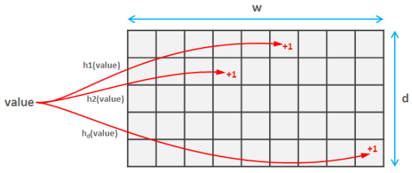
The basic idea of Count-Min Sketch [3] is quite simple and somehow similar to Linear Counting. Count-Min sketch is simply a two-dimensional array (d x w) of integer counters. When a value arrives, it is mapped to one position at each of d rows using d different and preferably independent hash functions. Counters on each position are incremented. This process is shown in the figure below:

It is clear that if sketch is large in comparison with the cardinality of the data set, almost each value will get an independent counter and estimation will precise. Nevertheless, this case is absolutely impractical – it is much better to simply maintain a dedicated counter for each value by using plain array or hash table. To cope with this issue, Count-Min algorithm estimates frequency of the given value as a minimum of the corresponding counters in each row because the estimation error is always positive (each occurrence of a value always increases its counters, but collisions can cause additional increments). A practical implementation of Count-Min sketch is provided in the following code snippet. It uses simple hash functions as it was suggested in [4]:

1 2 3 4 5 6 7 8 9 10 11 12 13 14 15 16 17 18 19 20 21 22 23 24 25 26 27 28 29 30 31 32

class CountMinSketch {     long estimators[][] = new long[d][w]    // d and w are design parameters     long a[] = new long[d]     long b[] = new long[d]     long p      // hashing parameter, a prime number. For example 2^31-1       void initializeHashes() {         for(i = 0; i < d; i++) {             a[i] = random(p)    // random in range 1..p             b[i] = random(p)         }     }       void add(value) {         for(i = 0; i < d; i++)             estimators[i][ hash(value, i) ]++     }       long estimateFrequency(value) {         long minimum = MAX_VALUE         for(i = 0; i < d; i++)             minimum = min(                 minimum,                 estimators[i][ hash(value, i) ]             )         return minimum     }       hash(value, i) {         return ((a[i] * value + b[i]) mod p) mod w     } }

Dependency between the sketch size and accuracy is shown in the table below. It is worth noting that width of the sketch limits the magnitude of the error and height (also called depth) controls the probability that estimation breaks through this limit:

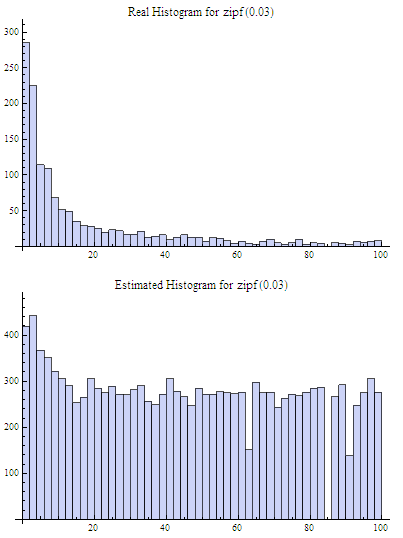
Accuracy of the Count-Min sketch depends on the ratio between the sketch size and the total number of registered events. This means that Count-Min technique provides significant memory gains only for skewed data, i.e. data where items have very different probabilities. This property is illustrated in the figures below.

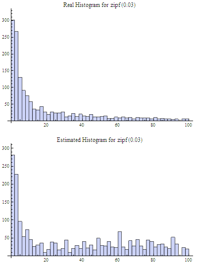
Two experiments were done with the Count-Min sketch of size 3×64, i.e. 192 counters total. In the first case the sketch was populated with moderately skewed data set of 10k elements, about 8500 distinct values (element frequencies follow Zipfian distribution which models, for example, distribution of words in natural texts). The real histogram (for most frequent elements, it has a long flat tail in the right that was truncated in this figure) and the histogram recovered from the sketch are shown in the figure below:

It is clear that Count-Min sketch cannot track frequencies of 8500 elements using only 192 counters in the case of low skew of the frequencies, so the estimated histogram is very inaccurate.

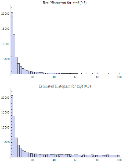
In the second case the sketch was populated with a relatively highly skewed data set of 80k elements, also about 8500 distinct values. The real and estimated histograms are presented in the figure below:

One can see that result is more accurate, at least for the most frequent items. In general, applicability of Count-Min sketches is not a straightforward question and the best thing that can be recommended is experimental evaluation of each particular case. Theoretical bounds of Count-Min sketch accuracy on skewed data and measurements on real data sets are provided in [6].

Frequency Estimation: Count-Mean-Min Sketch

The original Count-Min sketch performs well on highly skewed data, but on low or moderately skewed data it is not so efficient because of poor protection from the high number of hash collisions – Count-Min sketch simply selects minimal (less distorted) estimator. As an alternative, more careful correction can be done to compensate the noise caused by collisions. One possible correction algorithm was suggested in [5]. It estimates noise for each hash function as the average value of all counters in the row that correspond to this function (except counter that corresponds to the query itself), deduces it from the estimation for this hash function, and, finally, computes the median of the estimations for all hash functions. Having that the sum of all counters in the sketch row equals to the total number of the added elements, we obtain the following implementation:

1 2 3 4 5 6 7 8 9 10 11 12 13 14

class CountMeanMinSketch {     // initialization and addition procedures as in CountMinSketch     // n is total number of added elements       long estimateFrequency(value) {         long e[] = new long[d]         for(i = 0; i < d; i++) {             sketchCounter = estimators[i][ hash(value, i) ]             noiseEstimation = (n - sketchCounter) / (w - 1)             e[i] = sketchCounter – noiseEstimator         }         return median(e)     } }

This enhancement can significantly improve accuracy of the Count-Min structure. For example, compare the histograms below with the first histograms for Count-Min sketch (both techniques used a sketch of size 3×64 and 8500 elements were added to it):

Heavy Hitters: Count-Min Sketch

Count-Min sketches are applicable to the following problem: Find all elements in the data set with the frequencies greater than k percent of the total number of elements in the data set. The algorithm is straightforward:

• Maintain a standard Count-Min sketch during the scan of the data set and put all elements into it.
• Maintain a heap of top elements, initially empty, and a counter N of the total number of already process elements.
• For each element in the data set:
  • Put the element to the sketch
  • Estimate the frequency of the element using the sketch. If frequency is greater than a threshold (k*N), then put the element to the heap. Heap should be periodically or continuously cleaned up to remove elements that do not meet the threshold anymore.

In general, the top-k problem makes sense only for skewed data, so usage of Count-Min sketches is reasonable in this context.

Case Study

There is a system that tracks traffic by IP address and it is required to detect most traffic-intensive addresses. This problem can be solved using the algorithm described above, but the problem is not trivial because we need to track the total traffic for each address, not a frequency of items. Nevertheless, there is a simple solution – counters in the CountMinSketch implementation can be incremented not by 1, but by absolute amount of traffic for each observation (for example, size of IP packet if sketch is updated for each packet). In this case, sketch will track amounts of traffic for each address and a heap with the most traffic-intensive addresses can be maintained as described above.

Heavy Hitters: Stream-Summary

Count-Min Sketch and other similar techniques is not the only family of structures that allow one to estimate frequency-related metrics. Another large family of algorithms and structures that deal with frequency estimation is counter-based techniques. Stream-Summary algorithm [8] belongs to this family. Stream-Summary allows one to detect most frequent items in the dataset and estimate their frequencies with explicitly tracked estimation error.

Basically, Stream-Summary traces a fixed number (a number of slots) of elements that presumably are most frequent ones. If one of these elements occurs in the stream, the corresponding counter is increased. If a new, non-traced element appears, it replaces the least frequent traced element and this kicked out element become non-traced.

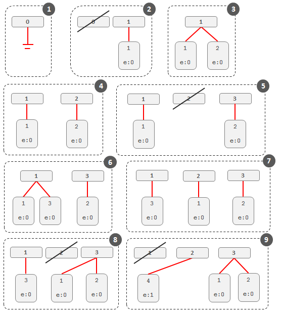
The figure below illustrates how Stream-Summary with 3 slots works for the input stream {1,2,2,2,3,1,1,4}. Stream-Summary groups all traced elements into buckets where each bucket corresponds to the particular frequency, i.e. to the number of occurrences. Additionally, each traced element has the “err” field that stores maximum potential error of the estimation.

1. Initially there is only 0-bucket and there is no elements attached to it.
2. Input : 1. A new bucket for frequency 1 is created and the element is attached to it. Potential error is 0.
3. Input : 2. The element is also attached to the bucket 1.
4. Input : 2. The corresponding slot is detached from bucket 1 and attached to the newly created bucket 2 (element 2 occurred twice).
5. Input : 2. The corresponding slot is detached from bucket 2 and attached to the newly created bucket 3. Bucket 2 is deleted because it is empty.
6. Input : 3. The element is attached to the bucket 1 because it is the first occurrence of 3.
7. Input : 1. The corresponding slot is moved to bucket 2 because this is the second occurrence of the element 1.
8. Input : 1. The corresponding slot is moved to bucket 3 because this is the third occurrence of the element 1.
9. Input : 4. The element 4 is not traced, so it kicks out element 3 and replaces it in the corresponding slot. The number of occurrences of the element 3 (which is 1) becomes a potential estimation error for the element 4. After this the corresponding slot is moved to the bucket 2, just like it was the second occurrence of the element 4.

The estimation procedure for most frequent elements and corresponding frequencies is quite obvious because of simple internal design of the Stream-Summary structure. Indeed, one just need to scan elements in the buckets that correspond to the highest frequencies. Nevertheless, Stream-Summary is able not only to provide estimates, but to answer are these estimates exact (guaranteed) or not. Computation of these guarantees is not trivial, corresponding algorithms are described in [8].

Range Query: Array of Count-Min Sketches

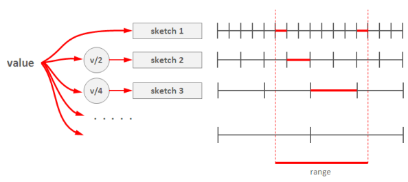
In theory, one can process a range query (something like SELECT count(v) WHERE v >= c1 AND v < c2) using a Count-Min sketch  enumerating all points within a range and summing estimates for corresponding frequencies. However, this approach is impractical because the number of points within a range can be very high and accuracy also tends to be inacceptable because of cumulative error of the sum. Nevertheless, it is possible to overcome these problems using multiple Count-Min sketches. The basic idea is to maintain a number of sketches with the different “resolution”, i.e. one sketch that counts frequencies for each value separately, one sketch that counts frequencies for pairs of values (to do this one can simply truncate a one bit of a value on the sketch’s input), one sketch with 4-items buckets and so on. The number of levels equals to logarithm of the maximum possible value. This schema is shown in the right part of the following picture:

Any range query can be reduced to a number of queries to the sketches of different level, as it shown in right part of the picture above. This approach (called dyadic ranges) allows one to reduce the number of computations and increase accuracy. An obvious optimization of this schema is to replace sketches by exact counters at the lowest levels where a number of buckets is small.

MADlib (a data mining library for PostgreSQL and Greenplum) implements this algorithm to process range queries and calculate percentiles on large data sets.

Membership Query: Bloom Filter

Bloom Filter is probably the most famous and widely used probabilistic data structure. There are multiple descriptions of the Bloom filter in the web, I provide a short overview here just for sake of completeness. Bloom filter is similar to Linear Counting, but it is designed to maintain an identity of each item rather than statistics. Similarly to Linear Counter, the Bloom filter maintains a bitset, but each value is mapped not to one, but to some fixed number of bits by using several independent hash functions. If the filter has a relatively large size in comparison with the number of distinct elements, each element has a relatively unique signature and it is possible to check a particular value – is it already registered in the bit set or not. If all the bits of the corresponding signature are ones then the answer is yes (with a certain probability, of course).

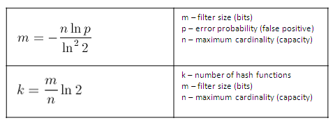
The following table contains formulas that allow one to calculate parameters of the Bloom filter as functions of error probability and capacity:

Bloom filter is widely used as a preliminary probabilistic test that allows one to reduce a number of exact checks. The following case study shows how the Bloom filter can be applied to the cardinality estimation.

Case Study

There is a system that tracks a huge number of web events and each event is marked by a number of tags including a user ID this event corresponds to. It is required to report a number of unique users that meet the specified combination of tags (like users from the city C that visited site A or site B).

A possible solution is to maintain a Bloom filter that tracks user IDs for each tag value and a Bloom filter that contains user IDs that correspond to the final result. A user ID from each incoming event is tested against the per-tag filters – does it satisfy the required combination of tags or not. If the user ID passes this test, it is additionally tested against the additional Bloom filter that corresponds to the report itself and, if passed, the final report counter is increased.

References

1. K. Whang, B. T. Vander-Zaden, H.M. Taylor. A Liner-Time Probabilistic Counting Algorithm for Database Applications
2. M. Durand and P. Flajolet. Loglog Counting of Large Cardinalities
3. G. Cormode, S. Muthukrishnan. An Improved Data Stream Summary: The Count-Min Sketch and its Applications
4. G. Cormode, S. Muthukrishnan. Approximating Data with the Count-Min Data Structure
5. F. Deng, D. Rafiei. New Estimation Algorithms for Streaming Data: Count-min Can Do More
6. G. Cormode, S. Muthukrishnan. Summarizing and Mining Skewed Data Streams
7. P. Flayjolet and N. Martin. Probabilistic counting algorithm for data base applications
8. A. Metwally, D. Agrawal, A.E. Abbadi. Efficient Computation of Frequent and Top-K Elements in Data Streams
9. P. Flayjolet, E.Fusy, O. Gandouet, F. Meunier. HyperLogLog: the analysis of a near-optimal cardinality estimation algorithm
10. P. Clifford, I. Cosma. A Statistical Analysis of Probabilistic Counting Algorithms